Understanding Excel Conditional Formatting

Conditional formatting is a feature in Microsoft Excel that allows you to apply formatting to a cell or a range of cells based on certain conditions or criteria. This means that you can change the color, font, or style of a cell depending on whether it meets a specific condition that you set. This is a powerful tool that can help you to visually highlight important data in your spreadsheet, track trends, and identify patterns.

Conditional formatting can be applied in several ways, such as by specific values, by formulas, or by rules. Each of these methods has its own benefits and limitations, depending on the type of data you are working with and the level of detail that you want to analyze. For example, you might use the “Highlight Cell Rules” option to change the font color of a cell if it exceeds a certain value, such as a budget threshold. Alternatively, you might use the “Data Bars” option to create a visual representation of the magnitude of a number, such as a progress bar or a thermometer.

The key advantage of conditional formatting is that it allows you to quickly and easily identify important information in your data by applying visual cues that are easy to recognize and understand. This can save you time and effort by helping you to focus on the most relevant data, rather than having to manually sift through large sets of data to find the information you need. Moreover, conditional formatting can be used to create dynamic dashboards, charts, and reports that update automatically as your data changes, making it a versatile tool for data analysis and visualization.

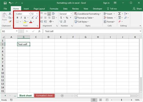
To apply conditional formatting to a cell or a range of cells in Excel, you can use the “Conditional Formatting” button in the “Home” tab of the ribbon. This will open a drop-down menu with several formatting options that you can choose from, including “Highlight Cells Rules”, “Color Scales”, “Data Bars”, “Icon Sets”, and “Conditional Formatting Rules Manager”. Each of these options has its own settings and parameters that you can customize to suit your needs. For example, if you want to highlight values that are above or below a certain threshold, you can use the “Highlight Cells Rules” option and select “Greater Than” or “Less Than” as your criteria.

Overall, conditional formatting is a powerful tool that can help you to gain insights from your data quickly and easily. By applying formatting based on certain criteria, you can create visual cues that highlight important information and make it easy to interpret and analyze your data. Whether you are using Excel for personal finance, data analysis, or business reporting, conditional formatting can be a valuable asset to help you make informed decisions and produce high-quality outputs.

Identifying the Target Cells for Blinking

When it comes to making a cell blink in Excel, the first step is to identify the target cells. These are the cells that you want to blink. The process of identifying the target cells for blinking may vary depending on the version of Excel that you are using. In general, however, there are a few common ways to do this.

The first method is to simply select the cells that you want to blink. To do this, click on the first cell that you want to blink and hold down the left mouse button. Then, drag the mouse over the cells that you want to include in the selection. Once you have selected all of the cells that you want to blink, you can move on to the next step.

Another option is to use a formula or function to identify the target cells. For example, you could use the =IF function to check a specific condition in each cell and return a value if the condition is met. You could then use conditional formatting to apply blink effects to the cells that meet the condition. This method requires some knowledge of Excel formulas and functions, but it can be very powerful once you master it.

Additionally, you may be able to use the built-in Name Manager in Excel to identify the target cells. This is useful if you have a large worksheet with many cells to blink. To use this method, you need to give a specific name to the cells that you want to blink. Then, you can use the Name Manager to search for cells with that name and apply blink effects to them.

Finally, you can use Visual Basic for Applications (VBA) to identify the target cells. VBA is a powerful programming language that is built into Excel. With VBA, you can write custom code to automate many tasks, including making cells blink. This method requires more advanced knowledge of programming, but it offers a lot of flexibility and customization.

Regardless of which method you choose, it is important to identify the target cells for blinking before you proceed. This will ensure that the blink effects are applied only to the cells that you want.

Setting Up the Conditional Formatting Rule for Blinking

Conditional formatting in Excel is a powerful feature that helps you to visually highlight the data based on specific criteria. One of the interesting things that you can do with it is to make your cell blink. In this article, we will show you how to make your cell blink in Excel without VBA using the Conditional Formatting Rule.

Step 1: Select the Cell(s) to Blink

The first step in making your cell(s) blink is to select the cell(s) that you want to highlight. You can select either a single cell or a range of cells. You can do this by clicking on a cell and dragging your mouse to select the cells or by using the keyboard shortcut Ctrl + Shift + Arrow keys to select a range of cells.

Step 2: Open the Conditional Formatting Dialog Box

Once you have selected the cell(s) to blink, the next step is to open the Conditional Formatting dialog box. You can do this by going to the Home tab, then clicking on the Conditional Formatting icon in the Styles group and selecting the New Rule option. Alternatively, you can use the keyboard shortcut Alt + H + L + N.

Step 3: Create the Conditional Formatting Rule

In the New Formatting Rule dialog box, select the “Use a formula to determine which cells to format” option. In the Format values where this formula is true box, enter the formula: =MOD(ROW(),2)=0. This formula checks whether the row number of the selected cell(s) is even. If it is, then the formula returns TRUE, it means that the cell is selected, and the formatting is applied. In the example below, the formula is applied to cell A1.

Note that you can modify the formula to suit your specific needs. For example, you can change the color of the blinking cell(s) or increase/decrease the speed of the blinking effect. You can also apply the formatting to specific rows or columns.

Step 4: Choose the Blinking Effect

Once you have created the conditional formatting rule, the next step is to choose the blinking effect. To do this, go to the Font tab in the Format Cells dialog box. Under Effects, check the “Blinking” option. You can also change the font color, style, and size if you want.

Click OK to apply the formatting to the selected cell(s). Now, when you move your mouse over the blinking cell(s), you will see that they blink in a fixed pattern with a default speed of 1 blink per second.

Finally, formatting options such as Font, Border, and Patterns can also be used to further customize the blinking effect. By experimenting with these formatting options, you can create a wide range of blinking effects that can make your spreadsheet more visually appealing and interactive.

Choosing the Appropriate Blink Speed

Using visual cues can help draw attention to specific pieces of data in an Excel spreadsheet. One of the easiest ways to do this is by using the blinking cell technique. This involves making a specific cell blink on and off repeatedly so that it’s more noticeable. If you’re looking to make a cell blink, it’s important to choose the right blink speed to ensure that the effect is effective. In this article, we’ll explore some of the factors that go into choosing the appropriate blink speed for your Excel sheet.

The first factor to consider when choosing the appropriate blink speed is the purpose of the blinking cell. Are you using it to highlight an important piece of data that requires immediate attention, or is it more of a secondary piece of information that should stand out but isn’t a top priority? Depending on the answer to this question, the blink speed can vary greatly.

If you’re looking to draw attention to critical information that requires immediate action, such as a deadline or an urgent task, a faster blink speed is recommended. This will make the cell more noticeable and ensure that the viewer doesn’t miss out on the important information. On the other hand, if you’re using the blinking cell to highlight less significant data, a slower blink speed is often more suitable.

Another factor to consider when choosing the speed of the blinking cell is the size of the spreadsheet. If you have a large sheet with lots of data, it may be necessary to slow down the blink speed to avoid overwhelming the viewer. If the blinking cell is the only highlighted piece of information on the sheet, a faster blink speed may be more appropriate since it’s easier to focus on a single point.

The intensity of the blinking cell is another factor to consider when deciding on the right blink speed. If the cell is blinking at a very fast rate, it may be too distracting and actually deter viewers from engaging with the data. Similarly, if the blinking cell is too slow, it may not be noticeable enough, resulting in the viewer overlooking the information entirely. It’s important to strike a balance between the blink speed and the intensity to achieve the most effective use of visual cues in Excel.

Finally, it’s essential to consider the audience when choosing the appropriate blink speed. A younger audience may be more receptive to faster blink speed, while older audiences may find it too distracting. Likewise, a professional setting may require a slower blink speed than a more casual one. Before settling on a particular blink speed, it’s essential to take into account the preferences of the audience.

Overall, choosing the appropriate blink speed for a cell in Excel involves considering several factors such as purpose, size of the data sheet, intensity of the blink, and audience preferences. With the right blink speed in place, you can effectively draw attention to the most important pieces of information in your Excel sheet.

Troubleshooting Common Issues with Blinking Cells in Excel

While blinking cells in Excel can add a dynamic element to your data, there are also common issues that can arise. Here are some troubleshooting tips:

1. Blinking cells are not flashing

If your cells are not flashing, check that the formatting options are set correctly. Select the cell and go to the Home tab. Then, click on the drop-down menu under the number formatting options and select “Custom.” In the Type field, enter this formula: “[Green][>0]✓;[Red][<=0]✓”. This formula will set up conditional formatting so that when the cell value is greater than 0, it will flash green, and when it is less than or equal to 0, it will flash red.

If the cell still isn’t flashing, try clicking “Format” and make sure that under the “Font” tab, the “Color” drop-down menu is set to “Automatic.”

2. Blinking cells are flashing inconsistently

If your cells are flashing inconsistently, it could be because the input values are not in the correct format. Check that all inputted values in the cell range are numbers and not text. You may also want to check that all cells that you are using in formulas or conditional formatting have the correct data types.

3. Blinking cells are slow to load

If your blinking cells are slow to load, it could be due to overly complicated formatting or too much data on the worksheet. Consider reducing the amount of information on the worksheet and simplifying formulas or conditional formatting.

4. Blinking cells disappear or stop flashing after copying or moving them

If you copy or move cells that are set to flash, the blinking may disappear. Check that the cells have not been accidentally moved or that the conditional formatting formula is still applying to the correct cell range. You may need to reapply the blinking formatting to the cell range after moving or copying if these actions break the conditional formatting formula.

5. Blinking cells are not printing or showing up in PDFs

Sometimes, blinking cells may not show up in print or in PDFs because the conditional formatting is not applied to the right range or the settings for the worksheet are incorrect. Check that the worksheet settings are set to “Print Active Sheets” and ensure that all cells that are set to blink are housed within the same worksheet. Try saving the worksheet as a PDF, and check that the blinking cells appear correctly.

By following these troubleshooting tips, you can have up-to-date and dynamic data that is easy to read and understand.